44 excel chart add data labels to all series

how to edit a legend in Excel — storytelling with data Click on your chart, and then click the "Format" tab in your Excel ribbon at the top of the window. From the very right of the ribbon, click "Format Pane.". Once that pane is open, click on the legend itself within your chart. In your Format Pane, the options will then look something like this: How to: Display and Format Data Labels - DevExpress When data changes, information in the data labels is updated automatically. If required, you can also display custom information in a label. Select the action you wish to perform. Add Data Labels to the Chart. Specify the Position of Data Labels. Apply Number Format to Data Labels. Create a Custom Label Entry.

Chart.ApplyDataLabels method (Excel) | Microsoft Docs Applies data labels to all the series in a chart. Syntax expression. ApplyDataLabels ( Type, LegendKey, AutoText, HasLeaderLines, ShowSeriesName, ShowCategoryName, ShowValue, ShowPercentage, ShowBubbleSize, Separator) expression A variable that represents a Chart object. Parameters Example

Excel chart add data labels to all series

How To Add Data Labels In Excel * English4room Click The Data Series You Want To Label. They Normally Come From The Source Data, But They Can Include Other Values As Well, As We'll See In In A Moment. Then Click The Chart Elements, And Check Data Labels, Then You Can Click The Arrow To Choose An Option About The Data Labels In The Sub Menu. Modifying Axis Scale Labels (Microsoft Excel) Follow these steps: Create your chart as you normally would. Double-click the axis you want to scale. You should see the Format Axis dialog box. (If double-clicking doesn't work, right-click the axis and choose Format Axis from the resulting Context menu.) Make sure the Number tab is displayed. (See Figure 1.) Add Vertical Lines To Excel Charts Like A Pro! [Guide] Once your chart has the additional chart series added, select the entire chart and navigate to the Chart Design tab in the Excel Ribbon. Select the Change Chart Type button to launch the Change Chart Type dialog box. Once the dialog box appears, click on the Combo menu item in the left-side pane.

Excel chart add data labels to all series. How to Add Axis Titles in a Microsoft Excel Chart Select your chart and then head to the Chart Design tab that displays. Click the Add Chart Element drop-down arrow and move your cursor to Axis Titles. In the pop-out menu, select "Primary Horizontal," "Primary Vertical," or both. If you're using Excel on Windows, you can also use the Chart Elements icon on the right of the chart. Excel Pie Chart Labels on Slices: Add, Show & Modify Factors The method to add category names to the data labels is given below step-by-step: 📌 Steps: First, double-click on the data labels on the pie chart. As a result, a side window called Format Data Labels will appear. Now, go to the drop-down of the Label Options to Label Options tab. Then, check the Category Name option. Excel - adding new data points to an existing chart When I right-click on one of the three series shown in my chart and then choosing "select data" the Select Data Source window which appears states that "the data range is too complex to be displayed". I would be most grateful if anyone could advise the next steps to take to display on my chart the additional data I have added to my table. Labels: How to: Display and Format Data Labels - DevExpress To display value labels, set the DataLabelBase.ShowValue property of the DataLabelOptions object to true. Series name. Series labels identify data series to which the data points in the chart belong. Most series include multiple data points, so the same name will be repeated for all data points in the series, which is probably overkill.

How To Show Two Sets of Data on One Graph in Excel Click the "Insert" tab and then look at the "Recommended Charts" in the charts group After you select the data, you can click the insert tab at the top of the spreadsheet to see the objects you can insert. In that tab, you can look at the charts group and find the "Recommended Charts" section to make a chart for your data. How To Add Data Labels In Excel } Esse 2022 You can add data labels to show the data point values from the excel sheet in the chart. Source: This will select "all" data labels. Select + sign in the top right of the graph; Typically A Chart Will Display Data Labels Based On The Underlying Source Data For The Chart. How can I get data labels to show for each column in a bar chart? Turn on 'Overflow text' under Data label' Format tab. Also, you can adjust the position of the Data Label by switching to 'Outside End' or 'Inside Center' so that your Data Label gets displayed properly. If this post helps, then mark it as 'Accept as Solution ' so that it could help others. Regards, Sanket Bhagwat Message 2 of 3 779 Views 0 Reply All About Chart Elements in Excel - Add, Delete, Change - Excel Unlocked To insert a chart, select this data and press the F11 function key ( for chart sheet ) or go to Clustered Column Chart > Charts Group > Insert Tab ( for embedded chart ). The following chart inserts. Click on the chart to activate it. On clicking the + icon you will see the entire list of chart elements with the checkboxes.

Label line chart series - Get Digital Help Double press with left mouse button on the cell that contains the data label. Put the prompt between the words. Press Alt + Enter. Press Enter. Back to top 3. Align data labels If you want the labels to be aligned to the left simply select the data label. Go to tab "Home" on the ribbon. Press with left mouse button on the "Align Left" button. How to Create a Mekko Chart (Marimekko) in Excel - Quick Guide Select the Label Marker series, right-click and choose 'Change Series Chart Type…' The 'Change Chart Type' dialog box will appear. From the series names, select the Label Marker and change the chart type to 'Line with Markers'. #10: Add and Format labels First, select the "Label Marker" series. Excel Chart VBA - 33 Examples For Mastering Charts in Excel VBA 2. Adding New Chart for Selected Data using Charts.Add Method : Creating Chart Sheet in Excel VBA. The following Excel Chart VBA Examples method will add new chart into new worksheet by default. You can specify a location to embedded in a particular worksheet. 'Here is the other method to add charts using Chart Object. How to set multiple series labels at once - Microsoft Tech Community Click anywhere in the chart. On the Chart Design tab of the ribbon, in the Data group, click Select Data. Click in the 'Chart data range' box. Select the range containing both the series names and the series values. Click OK. If this doesn't work, press Ctrl+Z to undo the change. Apr 09 2022 12:02 PM.

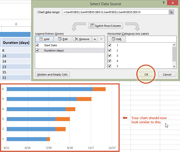
Gantt Chart Excel: Step-by-step, visual tutorial

How to Add Labels to Scatterplot Points in Excel - Statology Step 3: Add Labels to Points. Next, click anywhere on the chart until a green plus (+) sign appears in the top right corner. Then click Data Labels, then click More Options… In the Format Data Labels window that appears on the right of the screen, uncheck the box next to Y Value and check the box next to Value From Cells.

Directly Labeling Excel Charts - Policy Viz

How to Apply a Filter to a Chart in Microsoft Excel Select the chart and you'll see buttons display to the right. Click the Chart Filters button (funnel icon). When the filter box opens, select the Values tab at the top. You can then expand and filter by Series, Categories, or both. Simply check the options you want to view on the chart, then click "Apply."

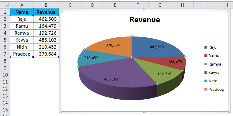
Pie Chart in Excel | How to Create Pie Chart | Step-by-Step Guide Chart

Openpyxl - Plotting Line Charts in Excel Code. import openpyxl from openpyxl.chart import Reference, LineChart, Series wb = openpyxl.load_workbook ('wb2.xlsx') sheet = wb.active # Data for plotting # Choose all the data from Column 2 to 4 values = Reference (sheet, min_col=2, max_col=4, min_row=1, max_row=11) # Create object of LineChart class chart = LineChart () chart.add_data ...

How to Change Excel Chart Data Labels to Custom Values? | Chandoo.org - Learn Microsoft Excel Online

Series.DataLabels method (Excel) | Microsoft Docs Example This example sets the data labels for series one on Chart1 to show their key, assuming that their values are visible when the example runs. VB Copy With Charts ("Chart1").SeriesCollection (1) .HasDataLabels = True With .DataLabels .ShowLegendKey = True .Type = xlValue End With End With Support and feedback

How to Add a Third Y-Axis to a Scatter Chart | EngineerExcel

How to add a single vertical bar to a Microsoft Excel line chart In the Chart Layouts group, click Add Chart Element. From the dropdown, choose Axes. From the resulting submenu, choose Secondary Vertical ( Figure J ), which displays the axes values to the right ...

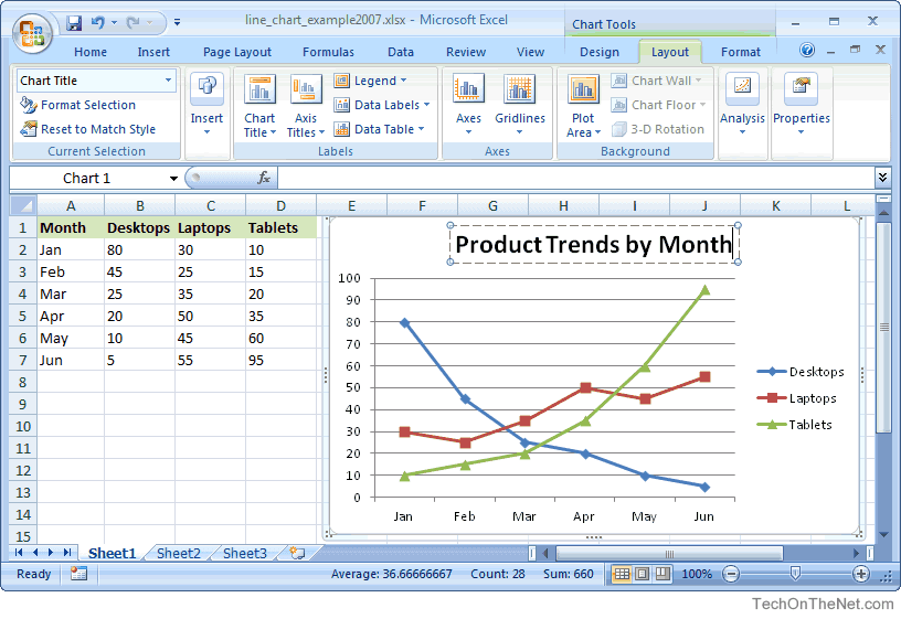
MS Excel 2007: How to Create a Line Chart

How to Make a Multi-Level Pie Chart in Excel (with Easy Steps) Step 5: Add Data Labels and Format Them. Adding data labels can help us analyze the information precisely. Right-click on the outermost level on the chart and then right-click on the chart. Then from the context menu, click on the Add Data Labels. After clicking on the Add Data Labels, the data labels will show accordingly.

"Waterfall" Chart in Microsoft Excel 2010

Bar Chart in Excel - Types, Insertion, Formatting To add Data Labels to the chart, perform the following steps:- Click on the Chart and go to the + icon at the top right corner of the chart. Mark the Data Labels from there After that, select the Horizontal Axis and press the delete key to delete the horizontal axis scale. This is how the chart looks once finished.

Step-by-step tutorial on creating clustered stacked column bar charts (for free) | Excel Help HQ

Excel Dynamic Chart Linked with a Drop-down List - GeeksforGeeks Follow the below steps to implement a dynamic chart linked with a drop-down menu in Excel: Step 1: Insert the data set into an Excel sheet in the cells as shown above. Step 2: Now select any cell where you want to create the drop-down list for the courses. Step 3: Now click on the Data tab from the top of the Excel window and then click on Data ...

Share :