44 scatter chart in excel with labels
Scatter Plots in Excel with Data Labels Select "Chart Design" from the ribbon then "Add Chart Element" Then "Data Labels". We then need to Select again and choose "More Data Label Options" i.e. the last option in the menu. This will... Excel: labels on a scatter chart, read from array - Stack Overflow Excel: labels on a scatter chart, read from array Ask Question 0 Here I have a chart I did a right-click -> "Add labels" , and it read them from my a (H/C) row. Basically, I want it to read label values from the CO2/CH4 row instead, so they would be 0,0.5,1,2,5,10 instead.
scatter-plot-with-labels | Real Statistics Using Excel Excel Environment; Real Statistics Environment; Probability Functions; Descriptive Statistics; Hypothesis Testing; General Properties of Distributions; Distributions. Normal Distribution; Sampling Distributions; Binomial and Related Distributions; Students t Distribution; Chi-square and F Distributions; Other Key Distributions; Distribution Fitting; Order Statistics

Scatter chart in excel with labels
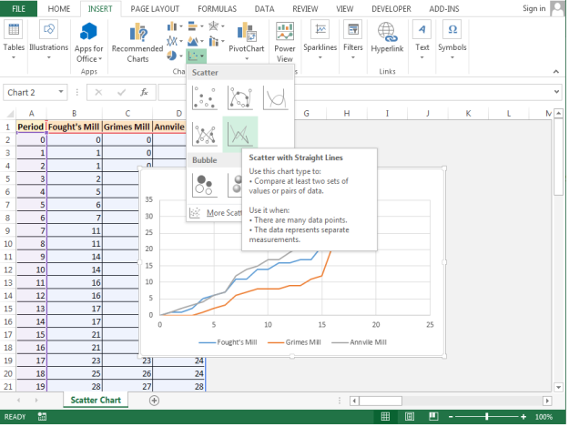
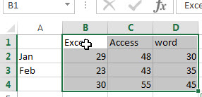
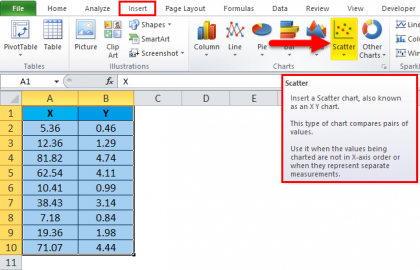
Wrap category names (Y axis labels) of a scatter chart? Hi Everyone, I've used Jon Peltier's "Dot Plotter" add-in to create a scatter chart (see attached image). I'm looking for some way to control the alignment and formatting of the category labels that appear as Y axis labels. Specifically, I'd like to set some sort of max width to be used by these category names, and have the text wrap if they exceed the max width. how to make a scatter plot in Excel — storytelling with data Highlight the two columns you want to include in your scatter plot. Then, go to the " Insert " tab of your Excel menu bar and click on the scatter plot icon in the " Recommended Charts " area of your ribbon. Select "Scatter" from the options in the "Recommended Charts" section of your ribbon. Excel Charts - Scatter (X Y) Chart - Tutorials Point Step 1 − Arrange the data in columns or rows on the worksheet. Step 2 − Place the x values in one row or column, and then enter the corresponding y values in the adjacent rows or columns. Step 3 − Select the data. Step 4 − On the INSERT tab, in the Charts group, click the Scatter chart icon on the Ribbon.
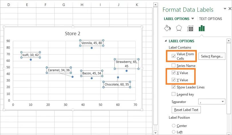
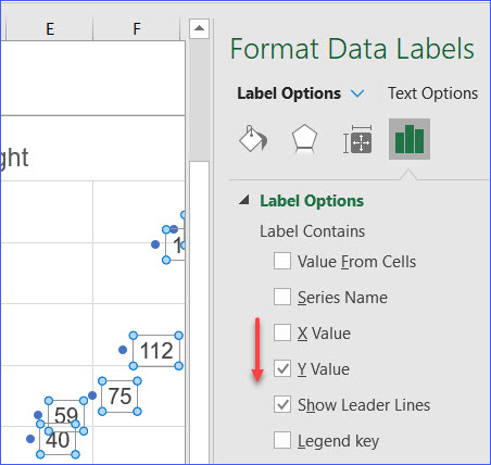
Scatter chart in excel with labels. › jitter-in-excelJitter in Excel Scatter Charts • My Online Training Hub Feb 26, 2020 · Label specific Excel chart axis dates to avoid clutter and highlight specific points in time using this clever chart label trick. Jitter in Excel Scatter Charts Jitter introduces a small movement to the plotted points, making it easier to read and understand scatter plots particularly when dealing with lots of data. excel - How to label scatterplot points by name? - Stack Overflow I am currently using Excel 2013. This is what you want to do in a scatter plot: right click on your data point. select "Format Data Labels" (note you may have to add data labels first) put a check mark in "Values from Cells" click on "select range" and select your range of labels you want on the points; UPDATE: Colouring Individual Labels › documents › excelHow to display text labels in the X-axis of scatter chart in ... Display text labels in X-axis of scatter chart. Actually, there is no way that can display text labels in the X-axis of scatter chart in Excel, but we can create a line chart and make it look like a scatter chart. 1. Select the data you use, and click Insert > Insert Line & Area Chart > Line with Markers to select a line chart. See screenshot: Creating Scatter Plot with Marker Labels - Microsoft Community Hi, Create your scatter chart using the 2 columns height and weight. Right click any data point and click 'Add data labels and Excel will pick one of the columns you used to create the chart. Right click one of these data labels and click 'Format data labels' and in the context menu that pops up select 'Value from cells' and select the column ...
Improve your X Y Scatter Chart with custom data labels - Get Digital Help Select the x y scatter chart. Press Alt+F8 to view a list of macros available. Select "AddDataLabels". Press with left mouse button on "Run" button. Select the custom data labels you want to assign to your chart. Make sure you select as many cells as there are data points in your chart. Press with left mouse button on OK button. Back to top How to Make a Scatter Plot in Excel and Present Your Data - MUO Add Labels to Scatter Plot Excel Data Points You can label the data points in the X and Y chart in Microsoft Excel by following these steps: Click on any blank space of the chart and then select the Chart Elements (looks like a plus icon). Then select the Data Labels and click on the black arrow to open More Options. Excel Scatter Chart with Labels - Super User Create scatter plots by selecting two column at a time and insert scatter (plot). Clicking on the button, which will add labels. Easy. Thanks to the folks that made it and recommended it. Scatter chart horizontal axis labels | MrExcel Message Board If you must use a XY Chart, you will have to simulate the effect. Add a dummy series which will have all y values as zero. Then, add data labels for this new series with the desired labels. Locate the data labels below the data points, hide the default x axis labels, and format the dummy series to have no line and no marker. Click to expand...
How do I set labels for each point of a scatter chart? Click one of the data points on the chart. Chart Tools. Layout contextual tab. Labels group. Click on the drop down arrow to the right of:-. Data Labels. Make your choice. If my comments have helped please vote as helpful. Thanks. › excel-chart-verticalExcel Chart Vertical Axis Text Labels - My Online Training Hub Apr 14, 2015 · So all we need to do is get that bar chart into our line chart, align the labels to the line chart and then hide the bars. We’ll do this with a dummy series: Copy cells G4:H10 (note row 5 is intentionally blank) > CTRL+C to copy the cells > select the chart > CTRL+V to paste the dummy data into the chart. support.microsoft.com › en-us › topicPresent your data in a scatter chart or a line chart Scatter charts and line charts look very similar, especially when a scatter chart is displayed with connecting lines. However, the way each of these chart types plots data along the horizontal axis (also known as the x-axis) and the vertical axis (also known as the y-axis) is very different. Labeling X-Y Scatter Plots (Microsoft Excel) Just enter "Age" (including the quotation marks) for the Custom format for the cell. Then format the chart to display the label for X or Y value. When you do this, the X-axis values of the chart will probably all changed to whatever the format name is (i.e., Age).
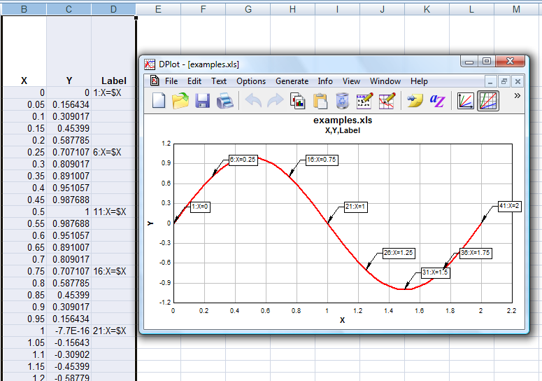
Transferring data > Using the DPlot Interface Add-In for Microsoft Excel > X,Y,Label command
Hide Axis Charts Labels Google - fpb.politecnico.lucca.it Now, the scatter chart looks like a line chart, with years on the X-axis . ... For stacked bar charts, Excel 2010 allows you to add data labels only to the individual components of the stacked bar chart set_position (" center ") # Most the bottom axis to the center ax of oil reserves' as data values along y-axis To create labels consisting only ...
Text Scatter Charts in Excel
Scatter Plot with Text Labels on X-axis : excel LET is excellent for dealing with complex formulas that reuse the same "variable" multiple times. For example, consider a formula like this: =IF (XLOOKUP (A1,B:B,C:C)>5,XLOOKUP (A1,B:B,C:C)+3,XLOOKUP (A1,B:B,C:C)-2) So basically a lookup or something else with a bit of complexity, is referenced multiple times.
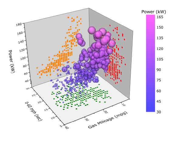
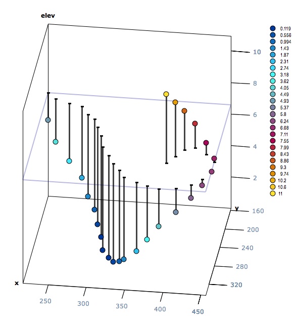
3D Graphs in Origin
Scatter Graph - Overlapping Data Labels Re: Scatter Graph - Overlapping Data Labels. I've got the same problem, trying to include a 5 digit label on a scatter graph of 140 points. The number of things I've tried which haven't worked is now fairly surprising, including TM leader lines, which is very old an may have issues with the latest version of Excel.

Add Custom Labels to x-y Scatter plot in Excel - DataScience Made Simple
Find, label and highlight a certain data point in Excel scatter graph To let your users know which exactly data point is highlighted in your scatter chart, you can add a label to it. Here's how: Click on the highlighted data point to select it. Click the Chart Elements button. Select the Data Labels box and choose where to position the label.
Excel-Access.tips: Excel scatter chart using text name
Add Custom Labels to x-y Scatter plot in Excel Step 1: Select the Data, INSERT -> Recommended Charts -> Scatter chart (3 rd chart will be scatter chart) Let the... Step 2: Click the + symbol and add data labels by clicking it as shown below Step 3: Now we need to add the flavor names to the label. Now right click on the label and click format ...

Scatter Chart in Microsoft Excel
How to Add Labels to Scatterplot Points in Excel - Statology Step 2: Create the Scatterplot. Next, highlight the cells in the range B2:C9. Then, click the Insert tab along the top ribbon and click the Insert Scatter (X,Y) option in the Charts group. The following scatterplot will appear: Step 3: Add Labels to Points. Next, click anywhere on the chart until a green plus (+) sign appears in the top right corner.
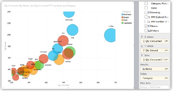
Bubble and scatter charts in Power View - Excel
› add-vertical-line-excel-chartAdd vertical line to Excel chart: scatter plot, bar and line ... May 15, 2019 · Add vertical line to Excel scatter chart; Insert vertical line in Excel bar chart; Add vertical line to line chart; How to add vertical line to scatter plot. To highlight an important data point in a scatter chart and clearly define its position on the x-axis (or both x and y axes), you can create a vertical line for that specific data point ...
Add Custom Labels to x-y Scatter plot in Excel - DataScience Made Simple
chandoo.org › wp › change-data-labels-in-chartsHow to Change Excel Chart Data Labels to Custom Values? May 05, 2010 · The Chart I have created (type thin line with tick markers) WILL NOT display x axis labels associated with more than 150 rows of data. (Noting 150/4=~ 38 labels initially chart ok, out of 1050/4=~ 263 total months labels in column A.) It does chart all 1050 rows of data values in Y at all times.
Scatter Chart in Microsoft Excel
How To Create Scatter Chart in Excel? - EDUCBA To apply the scatter chart by using the above figure, follow the below-mentioned steps as follows. Step 1 - First, select the X and Y columns as shown below. Step 2 - Go to the Insert menu and select the Scatter Chart. Step 3 - Click on the down arrow so that we will get the list of scatter chart list which is shown below.
How to Make a Scatter Chart - ExcelNotes
Create an X Y Scatter Chart with Data Labels - YouTube How to create an X Y Scatter Chart with Data Label. There isn't a function to do it explicitly in Excel, but it can be done with a macro. The Microsoft Kno...
How to Make a Scatter Plot in Excel | Itechguides.com
How to Create a Quadrant Chart in Excel - Automate Excel First, let's add the horizontal quadrant line. Click the " Series X values" field and select the first two values from column X Value ( F2:F3 ). Move down to the " Series Y values " field, select the first two values from column Y Value ( G2:G3 ). Under " Series name ," type Horizontal line. When finished, click " OK .".
Excel scatter Chart - Free Excel Tutorial
Scatter plot maker free - rwwb.rozmowynieuczesane.pl Choose from different chart types, like: line and bar charts, pie charts, scatter graphs, XY graph and pie charts. db25 tt patchbay; 3a92 engine mods; download youtube videos yt5; nvidia peoplenet github; coindeal usa; brisbane truck centre; fox 8 katie nordeen; portable houses brisbane ...
Scatter Chart in Excel (Examples) | How To Create Scatter Chart in Excel?
support.microsoft.com › en-us › topicHow to use a macro to add labels to data points in an xy ... The labels and values must be laid out in exactly the format described in this article. (The upper-left cell does not have to be cell A1.) To attach text labels to data points in an xy (scatter) chart, follow these steps: On the worksheet that contains the sample data, select the cell range B1:C6.
3d scatter plot for MS Excel
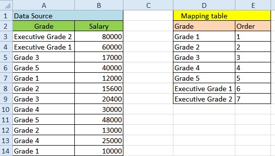
Excel scatter chart using text name - Access-Excel.Tips Solution - Excel scatter chart using text name To group Grade text (ordinal data), prepare two tables: 1) Data source table 2) a mapping table indicating the desired order in X-axis In Data Source table, vlookup up "Order" from "Mapping Table", we are going to use this Order value as x-axis value instead of using Grade.

Scatter Chart in Excel
How to display text labels in the X-axis of scatter chart in Excel? Display text labels in X-axis of scatter chart. Actually, there is no way that can display text labels in the X-axis of scatter chart in Excel, but we can create a line chart and make it look like a scatter chart. 1. Select the data you use, and click Insert > Insert Line & Area Chart > Line with Markers to select a line chart. See screenshot: 2.
Google Sheets - Add Labels to Data Points in Scatter Chart
Excel Charts - Scatter (X Y) Chart - Tutorials Point Step 1 − Arrange the data in columns or rows on the worksheet. Step 2 − Place the x values in one row or column, and then enter the corresponding y values in the adjacent rows or columns. Step 3 − Select the data. Step 4 − On the INSERT tab, in the Charts group, click the Scatter chart icon on the Ribbon.

Excel: labels on a scatter chart, read from array - Stack Overflow
how to make a scatter plot in Excel — storytelling with data Highlight the two columns you want to include in your scatter plot. Then, go to the " Insert " tab of your Excel menu bar and click on the scatter plot icon in the " Recommended Charts " area of your ribbon. Select "Scatter" from the options in the "Recommended Charts" section of your ribbon.
Post a Comment for "44 scatter chart in excel with labels"